Dropout: Why Throwing Half Your Network Away Makes It Generalise Better

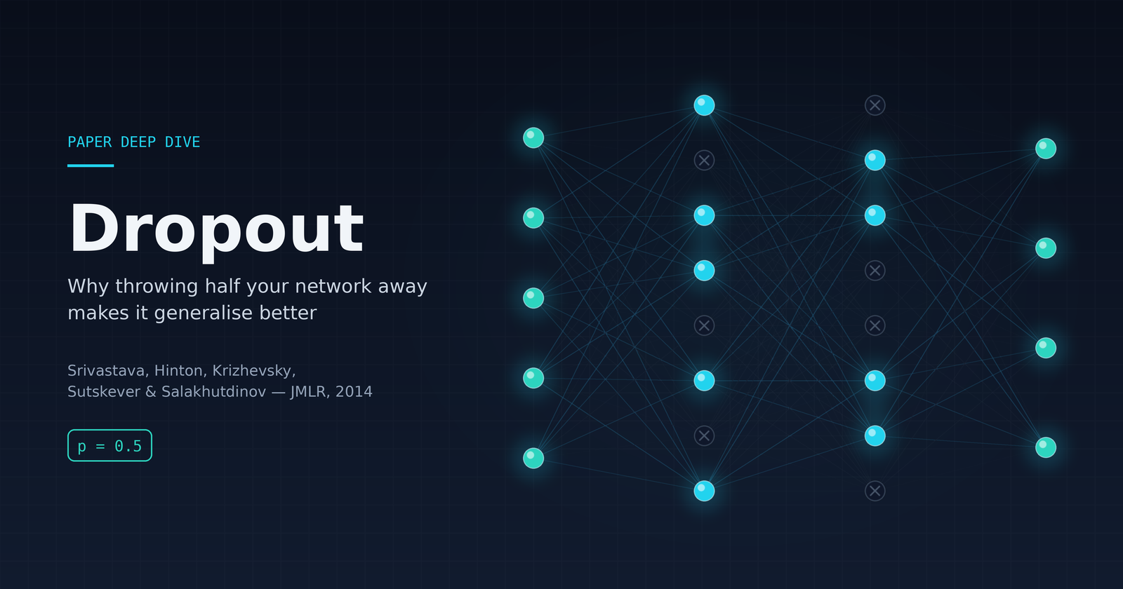
Some ideas in machine learning are clever. A few are almost insulting in how simple they are, and work anyway. Dropout is the second kind: during training, randomly delete half the units in your network, every single time you show it an example. Then, at test time, put them all back.

It sounds like sabotage. It won ImageNet.

The paper is Dropout: A Simple Way to Prevent Neural Networks from Overfitting by Nitish Srivastava, Geoffrey Hinton, Alex Krizhevsky, Ilya Sutskever and Ruslan Salakhutdinov, published in JMLR in 2014. It consolidates a technique that was already quietly powering the 2012 AlexNet result, and it is one of the most readable papers of the deep learning era. This post walks through what it actually says — the mechanism, the arithmetic, the evidence, and the practical guidance that is still worth following.

The problem: co-adaptation

A deep network with millions of parameters and 60,000 training images can learn essentially anything about that training set, including the noise. The standard framing is “overfitting”, but the paper offers a sharper diagnosis: co-adaptation.

In normal backpropagation, every parameter is updated to reduce the loss given what all the other units are currently doing. So a hidden unit is free to be sloppy, as long as another unit reliably cleans up after it. Over thousands of updates, units settle into brittle conspiracies: unit 47 only produces something useful when units 12 and 203 behave exactly as they did during training. That arrangement fits the training data beautifully and falls apart on data it has not seen.

The textbook fix is model averaging. Train ten different networks, average their predictions, and the idiosyncratic errors cancel out. It works reliably — and it is unaffordable. Ten large networks means ten times the training compute, ten times the hyperparameter search, ten times the inference cost, and you need enough data to train each one properly.

Dropout is a way to get the averaging without paying for it.

The idea

During training, each unit is retained with probability p, independently of the others, and dropped otherwise. Dropping a unit means temporarily removing it from the network along with all its incoming and outgoing connections. The paper’s default is p = 0.5 for hidden units and roughly p = 0.8 for input units.

Each training case therefore sees a different thinned network — a random sub-network sampled from the full one. A network with n units contains 2^n possible thinned networks, and they all share weights, so the total parameter count never changes. Training with dropout is, in the paper’s words, training a collection of 2^n thinned networks with extensive weight sharing, “where each thinned network gets trained very rarely, if at all”. With 2^n architectures and maybe a million weight updates, the overwhelming majority are never sampled even once — the weight sharing is doing all the work that would otherwise require 2^n separate models.

Two motivations run through the paper, and both are worth keeping in your head:

Evolution. Sexual reproduction breaks up co-adapted gene sets every generation, which looks like a bad deal for individual fitness — and yet it is how most complex organisms reproduce. One explanation is that selection optimises for mix-ability: a gene that only works alongside a specific set of partners is fragile, because those partners may not show up. A gene that does something useful on its own, or with a small number of collaborators, survives reshuffling. Dropout applies the same pressure to hidden units.

Conspiracies. Ten conspiracies of five people each are more likely to cause trouble than one conspiracy requiring fifty people to all play their parts correctly. A big conspiracy can work if conditions are stable and there is plenty of time to rehearse — that is the training set. Novel test data is not stable, and the large conspiracy fails.

What actually happens in the forward pass

For a standard network, layer l+1 computes:

z⁽ˡ⁺¹⁾ᵢ = wᵢ⁽ˡ⁺¹⁾ · y⁽ˡ⁾ + bᵢ⁽ˡ⁺¹⁾
y⁽ˡ⁺¹⁾ᵢ = f(z⁽ˡ⁺¹⁾ᵢ)

With dropout, one line is inserted:

r⁽ˡ⁾  ~ Bernoulli(p)          # one independent coin flip per unit
ỹ⁽ˡ⁾  = r⁽ˡ⁾ * y⁽ˡ⁾            # element-wise product
z⁽ˡ⁺¹⁾ᵢ = wᵢ⁽ˡ⁺¹⁾ · ỹ⁽ˡ⁾ + bᵢ⁽ˡ⁺¹⁾
y⁽ˡ⁺¹⁾ᵢ = f(z⁽ˡ⁺¹⁾ᵢ)

That is the entire modification. Backpropagation is unchanged — gradients flow only through the units that survived the mask, and a parameter that was dropped for a given training case simply contributes a zero gradient for that case. A fresh mask is sampled for every training case in every mini-batch.

The arithmetic of the test-time trick

Here is the part that deserves real attention, because it is where the ensemble interpretation gets cashed in.

At test time you cannot average the predictions of 2^n networks. The paper’s answer is almost embarrassingly cheap: use the full network, but multiply every outgoing weight by p. Let me show why that works with actual numbers before writing the expectation.

Take a single hidden unit with four incoming activations and four weights:

	unit 1	unit 2	unit 3	unit 4
activation y	2.0	1.0	3.0	0.5
weight w	0.5	−1.0	0.25	2.0

Without dropout, the pre-activation is:

z = (0.5)(2.0) + (−1.0)(1.0) + (0.25)(3.0) + (2.0)(0.5)
  = 1.0 − 1.0 + 0.75 + 1.0
  = 1.75

Now apply dropout with p = 0.5. There are 2⁴ = 16 possible masks, each equally likely. A few of them:

mask r	surviving terms	z
(1,1,1,1)	all	1.75
(0,0,1,1)	0.75 + 1.00	1.75
(1,1,0,1)	1.00 − 1.00 + 1.00	1.00
(0,0,1,0)	0.75	0.75
(0,0,0,0)	none	0.00

Average z over all 16 masks: 0.875. The spread is large — the standard deviation across masks is 0.94, so an individual thinned network’s answer is very noisy — but the mean is exactly half of 1.75.

Now the test-time network: keep every unit, but scale the weights by p = 0.5:

z = (0.25)(2.0) + (−0.5)(1.0) + (0.125)(3.0) + (1.0)(0.5)
  = 0.5 − 0.5 + 0.375 + 0.5
  = 0.875

Identical. And this is not a coincidence of the numbers chosen — it is just linearity of expectation:

E[z] = E[ Σᵢ rᵢ wᵢ yᵢ ] = Σᵢ E[rᵢ] wᵢ yᵢ = p · Σᵢ wᵢ yᵢ

Because rᵢ ~ Bernoulli(p) and E[rᵢ] = p, scaling the weights by p reproduces the expected pre-activation exactly. One forward pass through one network approximates the geometric-mean prediction of exponentially many thinned networks.

The approximation is exact only up to the nonlinearity f — the expectation of the pre-activation is preserved, not the expectation of the output. So the paper checks it empirically (§7.5): they sample k thinned networks per test case and average their predictions properly (Monte-Carlo averaging), then compare to the weight-scaling shortcut. Around k = 50 samples, Monte-Carlo catches up with weight scaling. Beyond that it is very slightly better, but well within one standard deviation. For a technique that costs one multiplication per weight, that is an excellent trade.

Note for practitioners: modern frameworks implement inverted dropout instead. Rather than scaling weights down by p at test time, they scale the surviving activations up by 1/p during training, leaving inference completely untouched. The two are equivalent (the paper points this out in §10), but inverted dropout means model.eval() does nothing but switch the mask off. This is why nn.Dropout(0.5) in PyTorch takes the drop probability, while the paper’s p is the retain probability — a sign-flip that has confused a great many people reading the paper and the docs side by side.

Why it works: two observable effects

The paper does not stop at the ensemble story. It looks at what dropout does to the network itself.

It breaks co-adaptation. Train two autoencoders on MNIST with 256 ReLU hidden units, one with dropout and one without, to similar reconstruction error, then visualise the first-layer features (Figure 7). Without dropout, the features are unstructured noise — no single unit detects anything meaningful, because meaning lives in the combination. With p = 0.5, the units turn into recognisable edge, stroke and spot detectors. Each unit has been forced to be useful on its own, because it cannot rely on any specific colleague being present.

It induces sparsity for free. As a side effect, and with no sparsity penalty anywhere in the loss, dropout drives activations toward zero. Mean activation of hidden units drops from about 2.0 without dropout to about 0.7 with it, and the activation histogram develops a sharp peak at zero with very few highly active units (Figure 8). Sparsity is normally something you pay for with an explicit KL or L1 term; here it arrives as a by-product.

What the benchmarks showed

The paper’s central empirical claim is that dropout improved generalisation on every dataset they tried, across vision, speech, text and genetics. Some of the headline numbers:

Dataset	Domain	Baseline without dropout	With dropout
MNIST (784-1024-1024-2048-10)	Vision	1.62% (same net, L2)	1.05% (dropout + max-norm)
SVHN (conv net)	Vision	3.95% (conv + max pooling)	2.55% (dropout in all layers)
CIFAR-10	Vision	14.98% (Snoek et al. tuned)	12.61%
CIFAR-100	Vision	43.48% (conv + max pooling, hand tuned)	37.20%
ImageNet ILSVRC-2010 (top-5)	Vision	25.7% (SIFT + Fisher vectors)	17.0% (conv net + dropout)
TIMIT (phone error)	Speech	23.4% (6-layer, no pretraining)	21.8% (6-layer)
Reuters-RCV1	Text	31.05%	29.62%

These are the paper’s own like-for-like comparisons, not “best result on the dataset” — a few dropout-free entries elsewhere in the tables beat the baseline column (max-norm alone reaches 1.35% on MNIST, stochastic pooling 42.51% on CIFAR-100, and a DBN-pretrained 8-layer net 20.7% on TIMIT).

A few observations that matter more than the raw numbers:

Dropout beats the other regularisers, and stacks with one of them. On the same MNIST architecture, L2 gives 1.62%, max-norm alone 1.35%, dropout + L2 1.25%, and dropout + max-norm 1.05%. Max-norm — constraining ‖w‖₂ ≤ c for each hidden unit’s incoming weight vector — is not decoration. It is what lets you run the very high learning rates that dropout needs without the weights exploding.

It helps in convolutional layers too, which surprised people. Conv layers have few parameters and were assumed not to overfit much. But adding dropout to the conv layers of the SVHN network on top of the fully-connected ones took error from 3.02% to 2.55%. The explanation the authors offer: dropout in the lower layers supplies noisy inputs to the higher fully-connected layers, which is where the overfitting lives.

The gain shrinks as data grows. The text result is the tell: Reuters-RCV1 has more than 200,000 training examples, and dropout buys only 31.05% → 29.62%. When overfitting is not the binding constraint, a regulariser has little to offer.

Where dropout does not help

This is the section most summaries skip, and it is the most useful one.

Very small datasets. The paper varies MNIST training set size from 100 to 50,000 examples with a fixed architecture (Figure 10). At 100 and 500 examples, dropout gives no improvement at all — in fact it is slightly worse. The model has enough capacity to overfit even through all that noise, and the noise just makes the fit worse. The benefit rises with dataset size, peaks, and then declines again as overfitting stops being a problem. There is a sweet spot: enough data that the network cannot memorise it despite the noise, not so much that it would not have overfitted anyway.

When a proper Bayesian treatment is affordable. On the Alternative Splicing genetics dataset (2,932 training examples), dropout improves a standard neural net from 440 to 567 bits of code quality — a real gain that beats PCA-based regression and SVMs — but a Bayesian neural network reaches 623. Dropout does equally-weighted model averaging; Bayesian networks weight each model by its posterior, which is the correct thing to do. When data is scarce and you can afford the compute, the correct thing wins.

Training time. A dropout network typically takes 2–3× longer to train than the same architecture without it. The gradients are extremely noisy, because each update is a gradient for a different random architecture rather than for the network you will eventually deploy. That noise is precisely what prevents overfitting, so it is a genuine trade-off, not an implementation detail to optimise away.

The practical guide (Appendix A)

The paper’s appendix is a compact tuning guide, and the heuristics in it hold up well.

Knob	Recommendation	Why
Layer width n	If n units is right without dropout, use at least n/p with it	Only pn units survive in expectation, so dropout reduces effective capacity. With p = 0.5, that means doubling the layer.
Learning rate	10–100× the rate that was optimal without dropout	Gradients are noisy and largely cancel each other out; you need bigger steps to make progress.
Momentum	0.95–0.99 (standard nets use ~0.9)	Same reason — averages out the gradient noise.
Max-norm constraint c	3 to 4	Keeps weights bounded so the aggressive learning rate and momentum cannot blow them up.
Retain probability p, hidden	0.5–0.8	Coupled to n: small p requires large n, which slows training and risks underfitting.
Retain probability p, input	~0.8	Inputs carry information you cannot regenerate; dropping 50% of them throws away too much.

The sensitivity analysis behind the p recommendation is worth knowing (Figure 9). With the architecture held fixed, test error is flat for 0.4 ≤ p ≤ 0.8 and rises sharply outside it — below 0.4 the network underfits (training error rises too), above 0.8 there is not enough noise to regularise. If instead you hold pn fixed — scaling the layer width so the expected number of surviving units stays constant — the curve is much flatter at low p, and the optimum sits near p = 0.6. Either way, 0.5 is a defensible default and the method is not fragile in this parameter.

One more variant the paper reports (§10): Gaussian dropout. Write the inverted form of standard dropout as multiplication by r_b, which takes the value 1/p with probability p and 0 otherwise — so E[r_b] = 1 and Var[r_b] = (1−p)/p. Gaussian dropout replaces that with r ~ N(1, σ²) where σ = √((1−p)/p), matching both moments exactly. No weight scaling is needed at test time, because the expectation is already 1. It performed slightly better — 0.95% vs 1.08% on MNIST, 12.5% vs 12.6% on CIFAR-10. Given identical first and second moments, the Gaussian is the highest-entropy choice and the Bernoulli the lowest; the authors note, carefully, that these preliminary results suggest the high-entropy case might work slightly better. It never caught on the way Bernoulli dropout did, but it is a clean idea.

Twelve years on

Dropout’s position has shifted. Batch normalisation, much larger datasets and heavy data augmentation have taken over most of the regularisation load in vision, and modern conv nets frequently use little or no dropout in convolutional layers. But the technique did not disappear — it moved. Transformer architectures apply dropout on attention weights, on residual connections and inside feed-forward blocks, typically at far gentler rates (drop probability 0.1 rather than 0.5). Wherever a model is large relative to its data, it is still one of the first things to reach for.

What has aged best is not the technique but the diagnosis. Co-adaptation — the idea that a model’s failure mode is brittle dependence between its parts, not simply “too many parameters” — reframed regularisation as something you do to a network’s internal structure rather than to the magnitude of its weights. That reframing outlived the specific fix.

Takeaways

• Dropout trains an ensemble of 2^n weight-sharing sub-networks at the cost of one network.
• At test time, scaling weights by p reproduces the expected pre-activation exactly — the whole ensemble approximated by a single forward pass. Modern frameworks do the equivalent scaling (1/p) during training instead.
• It works by breaking co-adaptation between units, which is visible directly in the learned features, and it produces sparse activations as a side effect.
• Use it when your model is large relative to your data. It gives nothing on very small datasets and little on very large ones.
• If you turn it on, widen your layers to roughly n/p, raise your learning rate by 10–100×, push momentum to 0.95–0.99, and add a max-norm constraint of 3–4. Dropout with default hyperparameters tuned for a non-dropout net will disappoint you.
• Budget 2–3× the training time.

---

Reference: Nitish Srivastava, Geoffrey Hinton, Alex Krizhevsky, Ilya Sutskever, Ruslan Salakhutdinov. Dropout: A Simple Way to Prevent Neural Networks from Overfitting. Journal of Machine Learning Research 15 (2014) 1929–1958. JMLR